




A gas sensor does not measure concentration directly in every design. It produces an electrical or optical response that must be interpreted using the sensor’s specified characteristics and a calibration relationship. A calibration curve describes how that response changes when the sensor is exposed to known concentrations of a target gas.
For engineers, the curve is more than a graph in a datasheet. It helps establish sensitivity, evaluate linearity, convert sensor output into concentration, identify response limitations, and assess whether a calibration model is suitable for the intended measurement range.
A simple sensor may have an approximately straight-line response over its rated range. Other technologies produce nonlinear responses and need a curve-fitting model, lookup table, or internal linearization. Environmental conditions, gas delivery, sensor aging, and measurement electronics can also change the relationship.
This guide explains how to interpret a gas sensor calibration curve, calculate slope and concentration, distinguish two-point from multipoint calibration, evaluate residual errors, and understand why different sensor technologies need different calibration methods.
Conceptual calibration curve showing the relationship between known gas concentration and sensor output. The plotted values are illustrative, not specifications for a particular sensor.
1. What Is a Gas Sensor Calibration Curve?
A gas sensor calibration curve is a mathematical or graphical relationship between a known gas concentration and the corresponding sensor response under defined test conditions.
The two axes are normally arranged as follows:
- X-axis: Target gas concentration, such as ppm, %vol, or %LEL.
- Y-axis: Sensor response, such as current, voltage, resistance, conductance, absorbance, or a digital output value.
The curve is established by exposing a sensor or measuring system to known concentrations and recording the output after the response has reached the required measurement condition.
A general calibration relationship can be written as:
[
Y=f(C)
]
Where:
- (Y) is the sensor output or response.
- (C) is the target gas concentration.
- (f(C)) is the calibration function for the defined sensor and operating conditions.
The calibration function may be linear or nonlinear. It may also be valid only over a specified concentration range, temperature range, humidity range, pressure range, and gas-flow condition.
Why is a calibration curve necessary?
The sensor’s raw output is not always expressed in ppm or %LEL. For example, an electrochemical sensing element may generate a current, while the instrument electronics convert that current into a voltage or digital count.
The calibration relationship allows the instrument to translate the measured signal into a concentration estimate. It also provides a way to assess whether the sensor response is sufficiently predictable for the intended application.
A calibration curve is useful for:
- Determining the relationship between sensor output and gas concentration.
- Calculating sensitivity or response slope.
- Establishing zero and span adjustments.
- Evaluating linearity and nonlinear behavior.
- Converting measured output into concentration.
- Identifying changes caused by aging or environmental conditions.
- Estimating calibration error and measurement uncertainty.
Calibration curve vs. calibration procedure
These terms are related but not interchangeable.
| Term | Meaning |
|---|---|
| Calibration curve | The relationship between known concentration and sensor response |
| Calibration procedure | The method used to expose, measure, adjust, and verify the instrument |
| Calibration model | The equation, coefficients, or lookup table used to represent the relationship |
| Calibration record | The stored test conditions, reference-gas values, measurements, adjustments, and results |
A curve can be generated during laboratory characterization, production testing, or field calibration. The required method depends on the sensor, instrument, accuracy target, and applicable safety or quality requirements.
2. Understanding Sensitivity and Calibration Curve Slope
Sensitivity describes how much the sensor response changes when gas concentration changes. When the calibration curve is plotted with sensor output on the Y-axis and concentration on the X-axis, sensitivity corresponds to the slope of the curve.
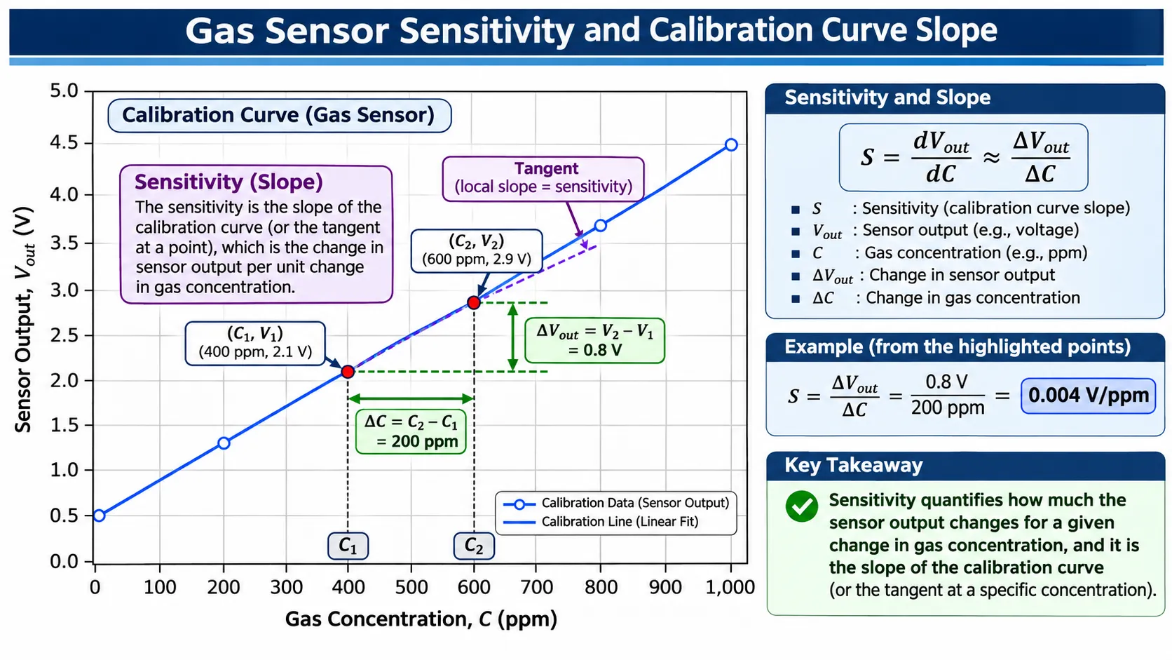
The slope represents the change in sensor output per unit change in gas concentration. The numerical values in this illustration are examples only.
Sensitivity for a linear calibration curve
For a linear response:
[
Y=mC+b
]
Where:
- (Y) is sensor output.
- (C) is gas concentration.
- (m) is the slope or sensitivity under this axis convention.
- (b) is the Y-axis intercept, often associated with the baseline or offset.
The slope can be calculated from two points:
[
m=\frac{\Delta Y}{\Delta C}
=\frac{Y_2-Y_1}{C_2-C_1}
]
For example, assume a sensor produces the following illustrative readings:
| Gas concentration | Sensor output |
|---|---|
| 20 ppm | 0.20 V |
| 60 ppm | 0.40 V |
The slope is:
[
m=\frac{0.40-0.20}{60-20}
=\frac{0.20}{40}
=0.005\ \mathrm{V/ppm}
]
This means the output changes by 5 mV for each 1 ppm increase in concentration over the illustrated interval.
The result is an example of output sensitivity. It is not a universal value for electrochemical, NDIR, MOS, catalytic, or PID sensors.
Common sensitivity units
The unit depends on the sensor’s output type and the concentration unit.
| Sensor output | Possible sensitivity unit |
|---|---|
| Electrochemical current | nA/ppm or µA/ppm |
| Analog voltage | mV/ppm or V/ppm |
| 4–20 mA transmitter | mA/ppm or mA per %LEL |
| Resistance | Ω/ppm, where a resistance-based response is appropriate |
| Conductance | S/ppm |
| Digital output | counts/ppm or digital units per concentration unit |
| NDIR optical response | Absorbance per concentration unit or a model-specific coefficient |
Always check the manufacturer’s definition. Some datasheets express sensitivity as output per concentration, while others use a different response convention.
Sensitivity in a nonlinear calibration curve
For a nonlinear response, the slope is not constant. The local sensitivity at a particular concentration is the derivative:
[
S(C)=\frac{dY}{dC}
]
This means a sensor may be more responsive to concentration changes in one part of its range than another.
For example, a sensor may show a steep response at low concentrations and a flatter response at higher concentrations as its output approaches saturation. In this case, reporting only one average slope can hide important behavior.
Does a higher slope mean a better sensor?
Not necessarily. A higher output slope can make small concentration changes easier to distinguish, but practical measurement performance also depends on noise, drift, repeatability, resolution, stability, usable range, and uncertainty.
A sensor with a high nominal sensitivity may still have poor low-concentration performance if its baseline noise or drift is also high.
For related concepts, see Gas Sensor Sensitivity vs Selectivity: What’s the Difference? and Signal-to-Noise Ratio in Gas Sensors: Why SNR Matters.
3. Linear vs. Nonlinear Gas Sensor Calibration Curves
Not every gas sensor has a straight-line relationship between concentration and output. The appropriate calibration model depends on the sensing principle, the sensor’s construction, the target gas, and the specified operating range.
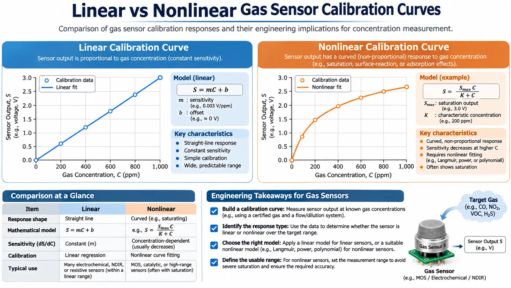
Conceptual comparison of linear and nonlinear responses. Real response shapes vary by sensor model and test conditions.
Linear response
A linear calibration curve can be represented by:
[
Y=mC+b
]
Within the validated range, a constant change in concentration produces an approximately constant change in output.
A linear model is useful because it is simple to calculate, store, verify, and implement in a microcontroller or transmitter.
Some electrochemical sensors are specified with an approximately linear current-to-concentration relationship over their recommended range. Other technologies can also be linearized over a defined range.
Nonlinear response
A nonlinear calibration curve cannot be adequately represented by one straight line across the full measurement range.
Possible models include:
- Polynomial regression.
- Power-law models.
- Exponential or logarithmic models.
- Physically based optical or electrochemical equations.
- Piecewise linear functions.
- Lookup tables with interpolation.
The model should be selected from measured data and supported by the sensor’s physical behavior. A high-order polynomial should not be chosen only because it produces a higher R² value.
Examples across sensor technologies
| Sensor technology | Calibration considerations |
|---|---|
| Electrochemical | Current is often approximately proportional to concentration over a specified range, but baseline, sensitivity, temperature, and sensor-specific behavior still matter |
| NDIR | Optical absorption is related to gas concentration, but detector output and the complete instrument response may require normalization and nonlinear linearization |
| MOS / semiconductor | Resistance or conductance often changes nonlinearly with gas concentration and environmental conditions |
| Catalytic bead | Bridge response may be approximately linear over a defined range, with deviations possible depending on concentration and operating conditions |
| PID | Ionization current can be related to concentration over a validated range; gas-specific response factors and instrument limits matter |
| Thermal conductivity | Output depends on the thermal properties of the gas mixture, so background-gas composition is important |
An NDIR example: calibration is not always a straight-line fit
Alphasense’s NDIR application note AAN 201-06 describes a method that uses active and reference detector signals to determine absorbance. The calculation includes a zero value, a span value, and linearization coefficients.
The note gives the following absorbance relationship:
[
ABS=1-\frac{ACT}{REF\times ZERO}
]
Where:
- (ACT) is the active-channel signal.
- (REF) is the reference-channel signal.
- (ZERO) is the normalized zero-gas reference value.
The gas concentration is then calculated using a nonlinear expression involving absorbance, span, and linearization coefficients. This is a specific Alphasense NDIR calculation method, not a universal formula for every NDIR sensor.
This example demonstrates why engineers should not assume that all gas sensor calibration curves can be represented by a simple linear equation.
4. Zero Calibration vs. Span Calibration
Zero and span calibration establish important reference points for a gas-measurement system. They are commonly used for instruments with a defined baseline and measurement range.
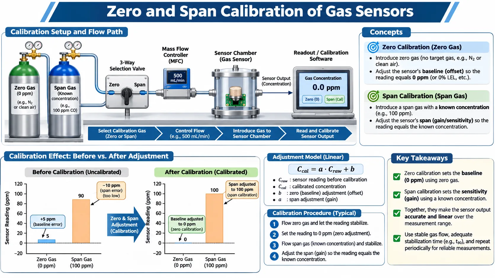
Conceptual zero- and span-calibration setup using a zero-gas source, a certified span-gas mixture, flow control, a sensor chamber, and calibration software.
What is zero calibration?
Zero calibration establishes the instrument’s baseline response under a defined zero-gas condition.
The zero gas should be appropriate for the sensor and application. It may be nitrogen, synthetic air, clean air, or another specified gas mixture. The correct choice depends on the target gas, sensor chemistry, background-gas requirements, and manufacturer’s instructions.
Zero calibration can be used to correct a baseline offset. It does not necessarily correct sensitivity or slope.
What is span calibration?
Span calibration uses a reference gas with a known target-gas concentration to adjust or verify the instrument response at a specified point.
The span-gas concentration should be suitable for the sensor’s measurement range and the manufacturer’s recommended calibration procedure.
A span adjustment may change the gain or sensitivity parameter so that the instrument reports the expected concentration at the reference point.
Zero and span are not the same as a full multipoint characterization
A zero point and one span point can be sufficient for a two-point linear adjustment when the sensor’s response is already known to be sufficiently linear over the intended range.
However, two points alone cannot demonstrate that the response is linear between or beyond those points. Additional concentrations are needed when the purpose is to characterize nonlinearity or validate a wider range.
A manufacturer-specific example
Honeywell’s 4 Series NDIR hydrocarbon characterization note describes a two-point user-calibration example using 0% LEL and 50% LEL reference gas for the sensor and gas types covered by that document.
The note also specifies a particular test arrangement and exposure condition. These details apply to that Honeywell sensor family and should not be treated as universal settings for all NDIR instruments.
Membrapor’s 2026 guidance for electrochemical gas sensors describes taking a baseline in fresh or synthetic air, exposing the sensor to a certified target-gas concentration, and waiting for a stable output before recording the calibration point. It recommends selecting a calibration concentration within a suitable part of the measurement range for the sensors covered by its guidance.
The practical lesson is to use the sensor manufacturer’s specified zero gas, span concentration, flow, stabilization time, and calibration sequence.
5. Two-Point vs. Multipoint Gas Sensor Calibration
Two-point calibration and multipoint calibration serve different purposes. The right choice depends on whether the response is already known to be linear and whether the goal is routine adjustment or full response characterization.
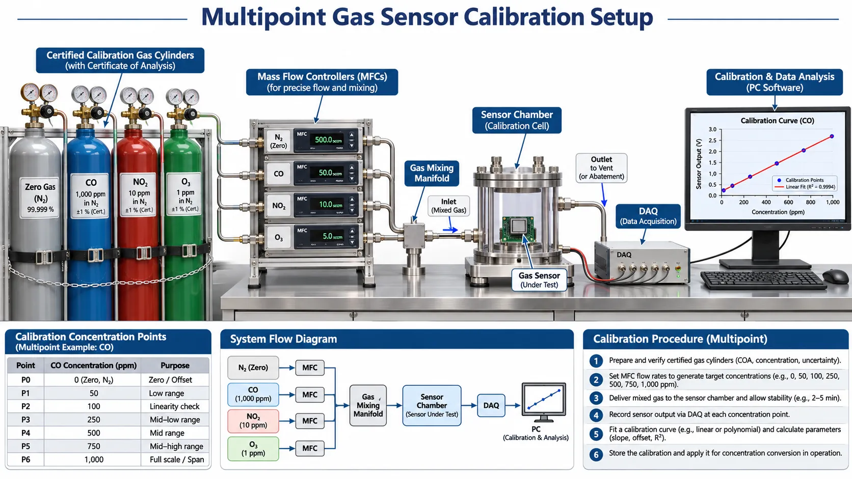
Illustrative laboratory setup with certified gas cylinders, mass flow controllers, a gas-mixing manifold, a sensor chamber, data acquisition, and calibration software.
Two-point calibration
A typical two-point linear calibration uses:
- A zero-gas point to establish the baseline.
- A known span-gas point to establish the response at a second concentration.
For a linear model, two points can determine the slope and intercept:
[
m=\frac{Y_2-Y_1}{C_2-C_1}
]
[
b=Y_1-mC_1
]
This method is practical when the sensor response is known to be linear within the required measurement range and the calibration procedure is validated.
Two-point calibration does not prove linearity. A sensor could match both calibration points but deviate between them.
Multipoint calibration
Multipoint calibration records sensor response at several known concentrations across the intended range.
A representative test plan might include:
| Point | Illustrative concentration | Purpose |
|---|---|---|
| P0 | 0 ppm | Baseline |
| P1 | 25 ppm | Low-range response |
| P2 | 50 ppm | Low-to-mid range |
| P3 | 100 ppm | Mid-range response |
| P4 | 150 ppm | Upper-mid range |
| P5 | 200 ppm | High-range response |
These are example concentrations only. Actual calibration points must be selected according to the sensor range, target application, certified gas availability, and manufacturer’s instructions.
Multipoint data can help engineers:
- Identify nonlinear response.
- Estimate slope across different parts of the range.
- Compare linear and nonlinear models.
- Detect saturation or an unsuitable operating range.
- Evaluate residuals and fit quality.
- Build a lookup table or compensation function.
How to build a multipoint calibration dataset
A practical laboratory workflow includes:
- Confirm the sensor model, rated range, and required operating conditions.
- Select suitable certified gas mixtures and verify their stated concentration and uncertainty.
- Prepare the zero-gas and target-gas delivery system.
- Use suitable flow-control and mixing equipment where dilution is required.
- Allow the sensor chamber and sensor output to stabilize at each concentration.
- Record the sensor output, gas concentration, temperature, humidity, pressure, and flow conditions.
- Repeat measurements where required to assess repeatability.
- Fit a suitable calibration model.
- Evaluate residuals and validate the model using independent measurements where possible.
- Store the calibration coefficients, test conditions, and traceable records.
For safety, gas cylinders, regulators, flow systems, exhaust arrangements, and exposure limits must be appropriate for the target gas. Toxic, corrosive, flammable, or oxygen-displacing gases require suitable engineering controls and trained personnel.
6. How to Calculate Gas Concentration from a Calibration Curve
Once a calibration model has been established, the instrument can use the measured sensor output to estimate gas concentration.
Concentration calculation for a linear curve
For a linear calibration relationship:
[
Y=mC+b
]
Rearrange the equation to calculate concentration:
[
C=\frac{Y-b}{m}
]
Where:
- (C) is the estimated gas concentration.
- (Y) is the measured sensor output.
- (m) is the calibration slope.
- (b) is the baseline or Y-intercept.
Worked example
Assume a hypothetical sensor has been characterized with the following linear model:
[
Y=0.005C+0.08
]
Here, (Y) is measured in volts and (C) is measured in ppm.
If the measured output is 0.73 V:
[
C=\frac{0.73-0.08}{0.005}
]
[
C=130\ \mathrm{ppm}
]
The estimated concentration is 130 ppm under the conditions represented by this illustrative calibration model.
The equation is an educational example. It is not a calibration specification for a commercial gas sensor.
Calculating concentration from a nonlinear curve
For a nonlinear calibration model:
[
Y=f(C)
]
The instrument must solve the inverse relationship:
[
C=f^{-1}(Y)
]
Depending on the model, this may involve an analytical equation, numerical calculation, interpolation, or a lookup table.
A lookup table is often useful for embedded systems because it can store measured calibration points and use interpolation between them. The interpolation method must be appropriate for the curve and validated over the intended range.
Why extrapolation is risky
A calibration equation should be used only within its validated range unless the manufacturer has established that extrapolation is acceptable.
A model that fits data from 0 to 200 ppm should not automatically be used to estimate 500 ppm. The sensor may become nonlinear, saturate, or operate outside its specified range.
For related concepts, see Gas Sensor Measurement Range vs Linear Range vs Overload.
7. How to Evaluate Calibration Curve Quality
A calibration curve should be assessed using more than its visual appearance or a single goodness-of-fit statistic. Engineers need to understand how closely the model represents the data and whether the remaining errors are acceptable for the application.
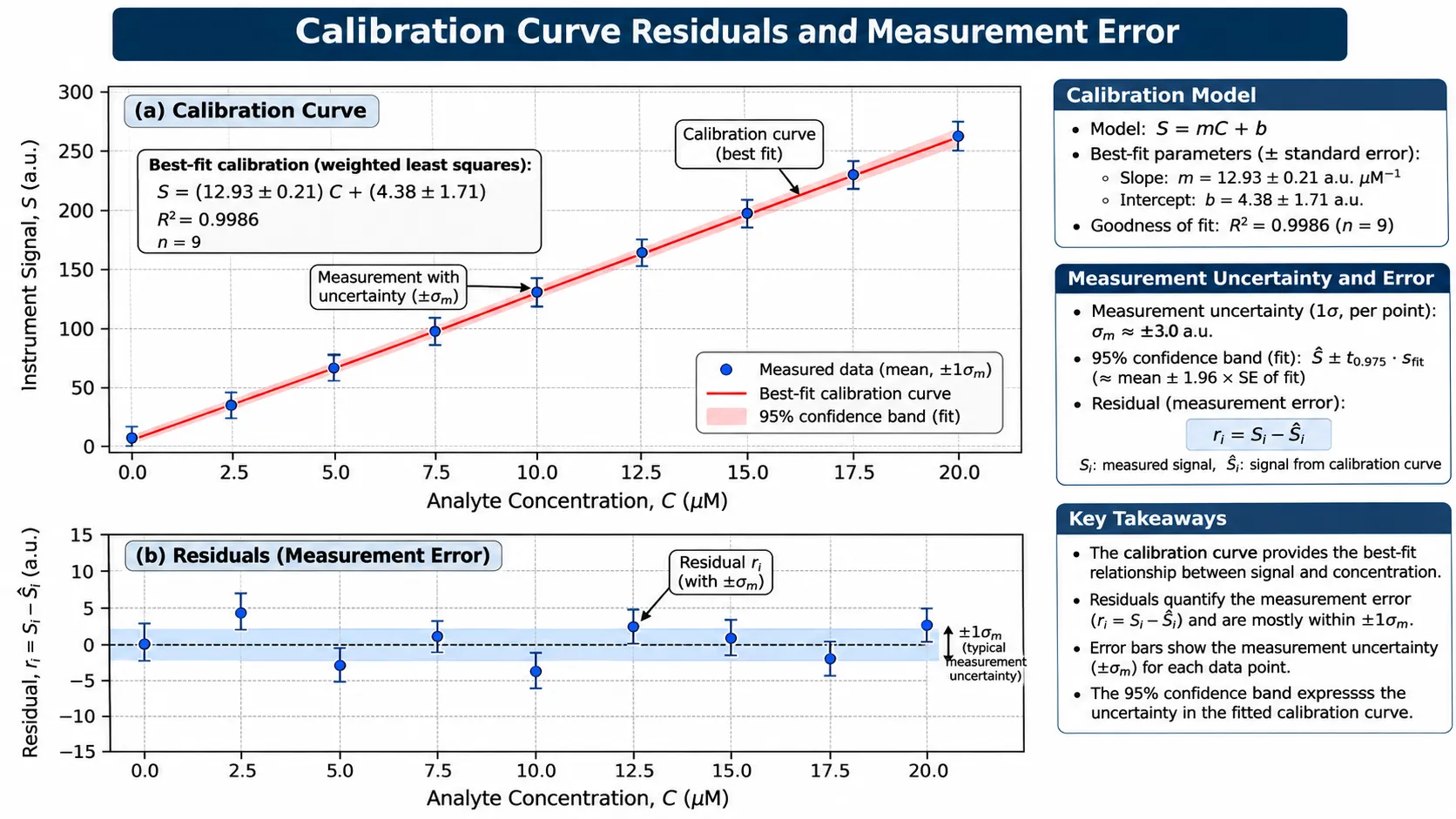
Illustrative calibration fit and residual plot. Residuals show the difference between measured output and the output predicted by the fitted calibration model.
R-squared (R²)
The coefficient of determination is commonly used to describe how much of the variation in the measured response is represented by the fitted model.
[
R^2=1-\frac{\sum_{i=1}^{n}(Y_i-\hat{Y}i)^2}
{\sum{i=1}^{n}(Y_i-\bar{Y})^2}
]
Where:
- (Y_i) is the measured sensor output.
- (\hat{Y}_i) is the output predicted by the fitted model.
- (\bar{Y}) is the mean measured output.
- (n) is the number of observations.
An R² value closer to 1 often indicates that the model explains a large proportion of the observed variation. However, a high R² does not prove that the calibration is accurate, unbiased, or suitable for the intended use.
A model can have a high R² while still showing systematic errors at low concentrations or near the upper end of the range.
Residual error
A residual is the difference between a measured response and the response predicted by the calibration model:
[
r_i=Y_i-\hat{Y}_i
]
Residuals help reveal whether the model consistently overestimates or underestimates the response in particular concentration regions.
A useful residual plot should be checked for:
- A random distribution around zero.
- Curved patterns that suggest an unsuitable linear model.
- Increasing spread at higher concentrations.
- Outliers that may indicate test or measurement problems.
- Clusters that may correspond to different test conditions.
Root mean square error (RMSE)
RMSE summarizes the typical size of the residuals in the same units as the measured output:
[
RMSE=\sqrt{\frac{1}{n}\sum_{i=1}^{n}(Y_i-\hat{Y}_i)^2}
]
A lower RMSE indicates a closer fit to the measured data in the response units used. RMSE should be interpreted in context: its value depends on the output scale and the concentration range.
Calibration fit is not the same as measurement uncertainty
A calibration curve describes a fitted relationship. The uncertainty of a reported concentration can also include:
- Certified reference-gas concentration uncertainty.
- Gas dilution and flow-control uncertainty.
- Repeatability of the sensor and measurement electronics.
- Temperature, humidity, pressure, and flow effects.
- Baseline drift and sensor aging.
- Model-fit uncertainty and residual behavior.
- ADC, amplifier, and reference-voltage errors.
For safety-critical or regulated applications, the complete measurement system and calibration procedure should be assessed against the applicable requirements. R² alone is not an accuracy specification.
For related concepts, see Gas Sensor Detection Limit: LOD vs Resolution vs Accuracy.
8. Calibration Curves Across Different Gas Sensor Technologies
Different sensing technologies convert gas exposure into different physical and electrical signals. As a result, their calibration curves and mathematical models are not interchangeable.
Electrochemical gas sensors
Electrochemical sensors commonly produce a current related to the target-gas reaction at the working electrode. Within a specified operating range, current may be approximately proportional to concentration.
Calibration therefore often involves recording the baseline current and the steady-state current at a known gas concentration. The slope may be expressed in nA/ppm or µA/ppm, depending on the sensor.
Temperature, humidity, bias conditions, cross-sensitivity, and sensor aging can affect the measured response. The manufacturer’s datasheet should define the applicable range and test conditions.
NDIR gas sensors
NDIR sensors use infrared absorption to determine gas concentration. Their calibration may involve active and reference optical channels, zero normalization, span calibration, and a model that converts absorbance into concentration.
The Beer-Lambert relationship provides a foundation for understanding optical absorption, but a complete commercial sensor may also need to account for optical geometry, detector characteristics, gas pressure, temperature, and signal processing.
Alphasense AAN 201-06 is a useful example of an NDIR concentration calculation that uses normalized active and reference signals together with span and linearization coefficients.
MOS and semiconductor gas sensors
Metal-oxide semiconductor sensors often show a nonlinear change in resistance or conductance when exposed to gas. Their response may depend on gas concentration, temperature, humidity, heater conditions, and the sensor’s previous exposure history.
A power-law or other nonlinear model may be appropriate for some devices, but the model must be determined and validated for the specific sensor.
Catalytic bead sensors
Catalytic bead sensors detect combustible gases through the heat generated by catalytic oxidation at an active element, commonly measured as a change in resistance within a bridge circuit.
The bridge output is calibrated against known gas concentrations. The usable response range, gas type, oxygen availability, and sensor condition all matter. Poisoning or inhibition can reduce response and change the calibration relationship.
PID sensors
Photoionization detectors measure an electrical response generated when suitable compounds are ionized by ultraviolet light. Calibration is commonly performed with a specified reference gas, and the response to other compounds may be expressed using gas-specific response factors.
A correction factor should not be treated as a replacement for direct calibration when the application requires higher accuracy and the target gas can be used safely and reliably.
Thermal conductivity sensors
Thermal conductivity sensors respond to differences in thermal conductivity between the sample gas and a reference or background gas. The calibration curve therefore depends on the gas mixture, not just the concentration of one component in isolation.
A calibration developed for one background gas may not remain valid when the background composition changes.
9. Factors That Affect Gas Sensor Calibration Curves
A calibration curve is valid only under the conditions for which it was established, or under conditions covered by a validated compensation method.
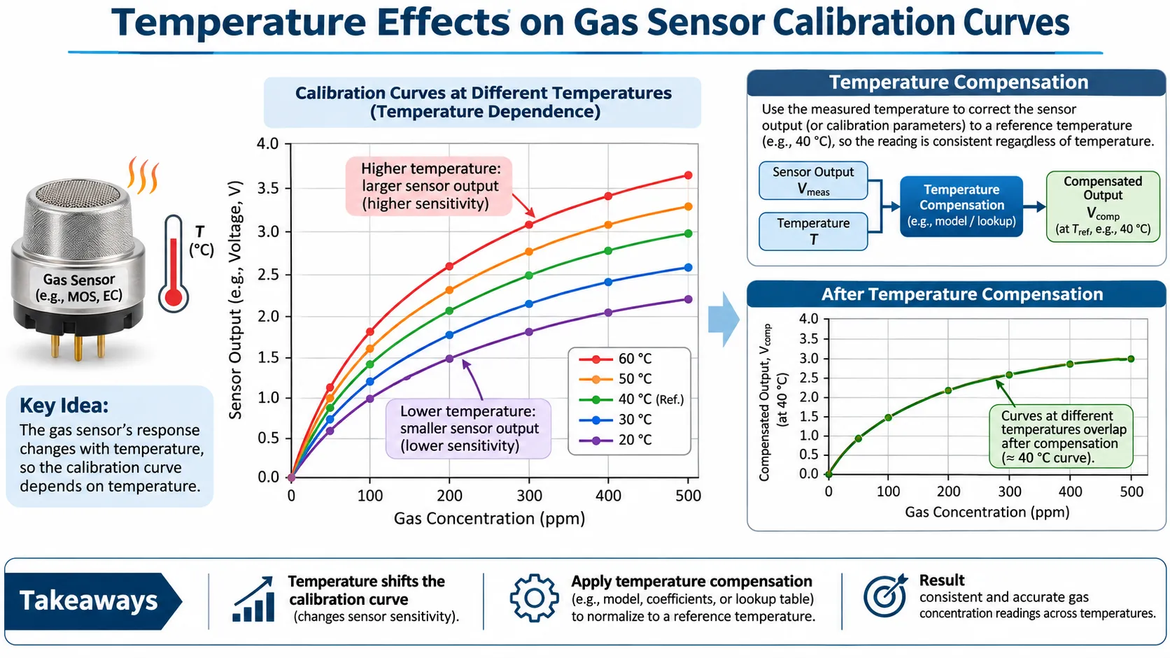
Illustrative comparison of calibration curves at different temperatures and a temperature-compensation concept. The direction and magnitude of temperature effects depend on the sensor technology and model.
Temperature
Temperature can affect the sensing reaction, diffusion, adsorption, optical components, electronics, and gas density. The direction and magnitude of the effect vary by sensing technology and sensor model.
Some instruments use temperature compensation coefficients, lookup tables, or multiple calibration curves to correct the response.
See How Temperature Affects Gas Sensor Readings.
Humidity
Humidity can affect electrolyte behavior, surface adsorption, gas diffusion, and the response of semiconductor materials. A calibration performed under very dry conditions may not represent performance in a humid application.
See How Humidity Affects Gas Sensors.
Pressure and gas flow
Pressure can change gas density and, for some technologies, the relationship between the measured signal and concentration. Flow rate and chamber design affect how quickly the target gas reaches the sensor and whether the test atmosphere is stable.
The calibration setup should reproduce the manufacturer’s recommended flow, pressure, and delivery arrangement.
Sensor aging and drift
Sensitivity and baseline can change over time. A calibration that was valid when the sensor was new may become less representative as the sensing element ages.
See Gas Sensor Stability vs Drift: What’s the Difference?.
Poisoning and cross-sensitivity
Interfering gases may produce additional response, while catalyst poisons or other contaminants may reduce sensor performance. These effects can alter the calibration relationship rather than simply adding a constant offset.
See Gas Sensor Poisoning vs Cross-Sensitivity.
Calibration gas and delivery accuracy
The reference concentration is only as reliable as the gas mixture and delivery system. Certified gas concentration, cylinder stability, regulator compatibility, dilution accuracy, tubing adsorption, leaks, and flow control can all contribute to uncertainty.
Use a gas mixture and delivery arrangement appropriate for the target gas and sensor. Record the reference-gas information and relevant test conditions.
10. Common Gas Sensor Calibration Curve Errors
Using inaccurate reference gas
If the actual gas concentration differs from the stated value, the calibration model will be based on incorrect reference data. Use suitable certified reference materials and follow their handling and shelf-life requirements.
Using too few calibration points
Two points can define a straight line, but they cannot reveal whether the sensor response is nonlinear between those points. Use multipoint characterization when the response shape or measurement range requires it.
Ignoring the zero offset
A non-zero baseline can cause a concentration calculation error if the model assumes that output is zero at zero concentration. Measure and account for the baseline using the specified procedure.
Fitting a linear model to nonlinear data
A straight-line fit may look acceptable over a limited region but produce large errors elsewhere. Inspect residuals and compare candidate models over the full intended range.
Ignoring environmental conditions
Temperature, humidity, pressure, and gas flow can change the response. Record these conditions and use compensation only where it has been validated.
Using calibration data outside the validated range
Do not extrapolate a calibration curve beyond its established range without evidence that the model remains valid.
Confusing a bump test with calibration
A bump test is generally a functional check that confirms the sensor or instrument responds to gas. It does not necessarily determine or verify the sensor’s sensitivity with calibration-level accuracy.
Membrapor’s 2026 guidance distinguishes function tests, quality-control measurements, and full calibration. Its discussion emphasizes that a function test can confirm a response without establishing the sensor’s sensitivity as accurately as a full calibration.
Treating a high R² as proof of accuracy
R² does not reveal every systematic error or uncertainty source. Check residuals, reference-gas uncertainty, repeatability, and independent verification results.
11. How Often Should a Gas Sensor Calibration Curve Be Checked?
There is no single recalibration interval that applies to every gas sensor or instrument.
The interval depends on:
- The sensor technology and model.
- The manufacturer’s recommended calibration interval.
- The stability and drift observed in service.
- Environmental and contamination exposure.
- The consequences of an incorrect reading.
- Applicable regulations, site procedures, and quality requirements.
- The results of previous calibration and verification records.
A field bump test, a calibration check, and a full calibration are different activities. Their frequency and acceptance criteria should be defined separately.
Membrapor’s 2026 guidance recommends annual recalibration for the electrochemical sensors and procedures discussed in that document. This is a manufacturer-specific recommendation, not a universal annual interval for every electrochemical sensor or gas detector.
For safety-related instruments, follow the manufacturer’s instructions, applicable standards, and the site’s documented gas-detection maintenance program.
12. Frequently Asked Questions
What is a gas sensor calibration curve?
A gas sensor calibration curve shows the relationship between known gas concentration and the corresponding sensor output under defined conditions. It is used to interpret sensor signals, calculate concentration, and evaluate response characteristics.
What does the slope of a calibration curve represent?
When sensor output is plotted on the Y-axis and gas concentration on the X-axis, the slope represents the change in output per unit change in concentration. For a linear curve, it is constant. For a nonlinear curve, local sensitivity changes with concentration.
Is sensitivity the same as calibration curve slope?
For the axis convention used in this article, sensitivity is the slope of the output-versus-concentration curve. In a nonlinear response, sensitivity is the local derivative at a particular concentration. Always check the manufacturer’s definition and units.
What is the difference between zero and span calibration?
Zero calibration establishes the baseline under a suitable zero-gas condition. Span calibration uses a known target-gas concentration to adjust or verify the response at a defined point. The exact gas mixtures and procedure depend on the sensor.
How many points are needed for gas sensor calibration?
Two points can determine the slope and intercept of a linear model. More points are needed to characterize nonlinear response, assess linearity across a range, or validate a more complex calibration model. The required number depends on the sensor and accuracy objective.
Why are some gas sensor calibration curves nonlinear?
The sensing mechanism, surface reactions, optical absorption, diffusion, gas-mixture properties, electronic processing, and saturation can all contribute to nonlinear behavior. The cause depends on the sensor technology and model.
How do you calculate gas concentration from sensor output?
For a linear model (Y=mC+b), calculate concentration using (C=(Y-b)/m). For a nonlinear model, use the validated inverse equation, numerical solution, or lookup table.
What is the difference between linearity and sensitivity?
Sensitivity describes how much the output changes for a concentration change. Linearity describes how closely the response follows a straight-line relationship over a defined range. A sensor can have high sensitivity but still show poor linearity.
How often should a gas sensor calibration curve be checked?
The interval depends on the sensor manufacturer’s recommendation, application risk, environmental conditions, observed drift, and applicable procedures. Do not apply one universal interval to all sensor technologies.
Does temperature affect gas sensor calibration?
Yes. Temperature can affect the sensing element, gas transport, optical components, and electronics. The direction and magnitude are sensor-dependent, so compensation should be based on manufacturer data or validated measurements.
Conclusion
A gas sensor calibration curve connects a known gas concentration to the sensor’s measured response. Its slope describes sensitivity, its intercept represents the baseline under the chosen model, and its shape indicates whether a linear or nonlinear calculation is appropriate.
For a reliable calibration:
- Use suitable certified reference gas and a controlled delivery system.
- Establish the baseline using the specified zero-gas procedure.
- Select calibration points across the intended measurement range.
- Use a linear model only where the response has been shown to be sufficiently linear.
- Evaluate residuals and uncertainty rather than relying on R² alone.
- Account for temperature, humidity, pressure, flow, aging, and interfering gases.
- Keep calibration records and follow the manufacturer’s verification and recalibration guidance.
The best calibration curve is not simply the one with the highest R². It is the model that represents the sensor accurately over the intended operating range, under defined conditions, with errors and uncertainty appropriate for the application.
References and Further Reading
Manufacturer technical references
- Alphasense — Application Note AAN 201-06: NDIR Gas Concentration Calculation Overview. Describes active/reference channel normalization, absorbance, span calibration, and nonlinear concentration calculation for the covered NDIR sensors.
- Honeywell — 4 Series NDIR Hydrocarbon Sensor: Sensitivity to Hydrocarbons Characterization Note. Provides a sensor-family-specific test and calibration example, including zero and span points.
- Membrapor — MEMPAPER Q3 2026: Quality Control, Calibration and Function Tests of Electrochemical Gas Sensors. Discusses the difference between function tests, quality control, and full calibration, along with baseline, sensitivity, stabilization, certified gas, and recalibration considerations.
- Membrapor — Application Note MEM1: Basics of Electrochemical Gas Sensors. Provides background on electrochemical gas-sensor operation and practical use.
- Membrapor — Technical Support and Application Notes. Manufacturer guidance and application-note resources.
Related GasNose articles
- Gas Sensor Sensitivity vs Selectivity: What’s the Difference?
- Gas Sensor Linearity and Linear Range Explained
- Gas Sensor Measurement Range vs Linear Range vs Overload
- Gas Sensor Detection Limit: LOD vs Resolution vs Accuracy
- Signal-to-Noise Ratio in Gas Sensors: Why SNR Matters
- Gas Sensor Stability vs Drift: What’s the Difference?
- How Temperature Affects Gas Sensor Readings
- How Humidity Affects Gas Sensors
